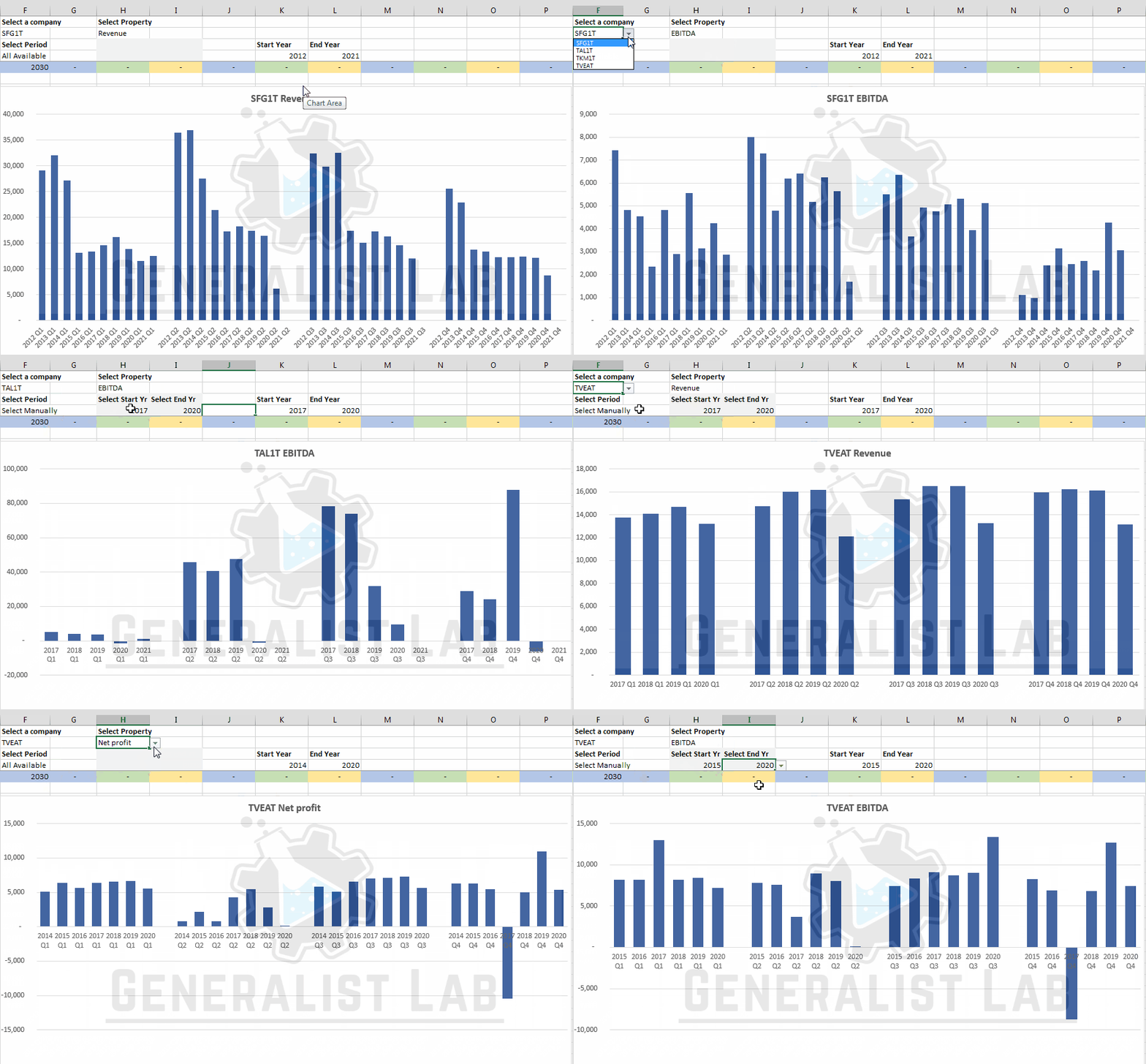
Two years ago I had a puzzle of automating some of my Excel charts. I could’t find a tutorial on how to create financial quarterly column charts based on dynamic cell references. So in last few days my first tutorial was born. By the end of it, you should be able to build this:

Along the way we will learn how to use some less known Excel functions as INDIRECT, INDEX, MATCH, OFFSET, NUMBERVALUE, COUNTIF functions and finally use Named Ranges to tie it all together in working dynamic chart controlled by dropdown selections you see above.
There’s a link to workbook free to download at the end of this how-to.
Dynamic Quarterly Charts: Problem Description
Say we have a company stock screener in Excel and want to plot quarterly financial data based on user selections. Here’s what we have to begin with:
- 4 companies data in individual sheets;
- each sheet has three parameters: revenue, net profit and EBITDA;
- Available historic data varies for each company. Some have data since 2012, others since 2015.
The task is to create a single dynamic chart, with flexible dates, company (data sourcing) and desired parameter to plot (revenue, net profit, EBITDA). How does one go about creating that chart from this mess?
Start: Where is Raw Data?
In my original problem, data was in a single sheet stacked vertically, but I figure more likely data distribution would be across sheets.
Important note: data is sequential. Date labels correspond to time, not data itself. For example 2015 Q3 corresponds to 2015.09.30, but revenue, net profit, EBITDA is for 9 months of 2015 (Q1+Q2+Q3) – for easier primary data entry be it manual or automatic.
So we have 4 company (named after ticker) specific sheets. Below is the sample image from two source data sheets.

Reserved place is up to 2030 Q4 and could easily be extended. So a next natural step would be to create a place bring it to one place.
Creating a master sheet
Sourcing Data
This step is not strictly necessary, but it will greatly help to shorten final formulas and avoid jumping around company specific sheets.
I created a hard-coded dropdown and dynamic text in A1 corresponding to dropdown selection.

Also we bring blank, formatted template with minimum data range found in all company sheets (2012).
Time to write some formulas to dynamically populate target company source data.
Since we have same column structure data in each of the sheets starts at the same row we only have to deal with two things: source sheet dependence and rows (date) variability across sheets. Let’s leave sheet dynamics aside for a while and implement simple index – match.
Bringing Data from Static Sheet with Index-Match
Even though we have picked TKM1T, let’s hardcode and source SFG1T sheet data first with formula ready to copy to rest of array in B3 cell:
=INDEX(SFG1T!$A$1:$D$200 ; MATCH($A3;SFG1T!$A:$A;0) ; MATCH(B$2;SFG1T!$1:$1;0))

First argument in Index formula is an array for source data. Fixing it’s coordinates and giving some space for future extension: up to 200 rows makes it:
SFG1T!$A$1:$D$200
We could of course dymanically calculate used range boundaries, but let’s stick to our primary task.
Second argument is a target row. Here match formula comes in, where we define which row is data label on in target sheet:
MATCH($A3;SFG1T!$A:$A;0)
And finally target column:
MATCH(B$2;SFG1T!$1:$1;0)
In all of the above, appropriate cell coordinates fixing is crucial in order to correctly copy formulas throughout whole date (2012-2030) and parameter (B-D columns) range.
Adding Source Sheet Dependence
INDIRECT formulas are messy in their syntax, but are very useful in their ability to change sheet and cell references dynamically. Simple example of INDIRECT formula usage:
=INDIRECT(F$2&"!$G$2") -> =SFG1T!$G$2
which brings SFG1T sheet G2 cell value into our target cell in our master sheet. SFG1T here is supplied from F2 cell value in master sheet. So B3 formula read to copy becomes:
=INDEX(INDIRECT($F$2&"!$A$1:$D$200") ; MATCH($A3;INDIRECT($F$2&"!$A:$A");0) ; MATCH(B$2;INDIRECT($F$2&"!$1:$1");0))
Effectively replacing hardcoded sheet name with fixed F2 cell reference. And we have data sourcing working.

Later we will introduce date range limits to handle #N/A data.
Calculating Quarterly Figures
As mentioned previously, currently we have 3, 6, 9 and 12 month figures. To start charting quarterly data we need to calculate it first.
Let’s form another table.

Formulas for Q1, Q2, Q3 and Q4 are all different, but let’s bring in 2021 Q1 revenues first from the table on the left with simple index-match.
=INDEX($B$3:$D$78 ; MATCH($F9&" "&G$6;$A$3:$A$78;0) ; MATCH(G$7;$B$2:$D$2;0))
We are sourcing data from fixed $B$3:$D$78 range, we need row to correspond date and quarter, so we built query from year and current quarter:
$F9 & " " G$6
and search in fixed green array $A$3:$A$78. Similarly for header column in orange array $B$2:$D$2.
For Q2 we perform a similar data retrieval, but finally subtract Q1:
=INDEX($B$3:$D$78 ; MATCH($F9&" "&J$6;$A$3:$A$78;0) ; MATCH(J$7;$B$2:$D$2;0))-G9
For Q3 we fetch 9M figure, and subtract Q1, Q2:
=INDEX($B$3:$D$78 ; MATCH($F9&" "&J$6;$A$3:$A$78;0) ; MATCH(J$7;$B$2:$D$2;0))-J9-G9
Similarly for Q4 we fetch 12 months figure, and subtract Q1, Q2, Q3 quarterly figures:
=INDEX($B$3:$D$78 ; MATCH($F9&" "&J$6;$A$3:$A$78;0) ; MATCH(J$7;$B$2:$D$2;0))-M9-J9-G9
Corrections for Incomplete Year Data
Say we have SFG1T financial data for 2021 Q1. Our current formula copied to rest of table would produce negative Q2 financial data, because there’s no half year data (2021 Q2) and Q2 is being calculated as Q2 = 6M – Q1.
We only need to correct for Q2, Q3 and Q4. So the corrective logic for Q2 to implement would be:
If fetched Q2 (6 months) data is empty (=0), then 0, else, fetch Q2 and calculate real Q2 financials. For cell J9 formula becomes:
=IF( INDEX($B$3:$D$78;MATCH($F9&" "&J$6;$A$3:$A$78;0);MATCH(J$7;$B$2:$D$2;0))=0 ; 0 ; INDEX($B$3:$D$78;MATCH($F9&" "&J$6;$A$3:$A$78;0);MATCH(J$7;$B$2:$D$2;0))-G9)
Similarly for Q3 logic: if fetched 9M figure = 0 then Q3=0, else fetched Q3 = 9M – Q2 – Q1. Cell M9 formula:
=IF(INDEX($B$3:$D$78;MATCH($F9&" "&M$6;$A$3:$A$78;0) ; MATCH(M$7;$B$2:$D$2;0))=0 ; 0 ; INDEX($B$3:$D$78;MATCH($F9&" "&M$6;$A$3:$A$78;0);MATCH(M$7;$B$2:$D$2;0))-J9-G9)
And finally for Q4, similarly in P9 cell:
=IF(INDEX($B$3:$D$78;MATCH($F9&" "&P$6;$A$3:$A$78;0);MATCH(P$7;$B$2:$D$2;0))=0 ; 0 ; INDEX($B$3:$D$78;MATCH($F9&" "&P$6;$A$3:$A$78;0);MATCH(P$7;$B$2:$D$2;0))-M9-J9-G9)
Now we are ready to populate rest of the table copying crafted formulas for each quarter columns and then the rest of years, which concludes the easy part.

Building blocks to Plot Quarterly Data
Static Chart Data Format
Let’s start without any automation first, just to get something to work on. We need stacked quarterly data with a single row left blank to separate individual quarter groups. Let’s do just that for now:

That’s a bunch of copied values and prepared date (x axis) series. Nothing dynamic so far, but we have a clear image of what our data should look like to form a target column chart.
Setting Chart Title as Cell Reference
A little side note, let’s add dynamic chart title tied to cell reference:

Now let’s start with crafting X axis.
Building Block: All Possible X Axis Values
Naturally we must be thinking of corner cases and start with minimum and maximum years (2012-2030). So we stack all possible years in similar fashion we did previously.

Formula references are not necessary, but helps avoid typos. Next we need to dynamically change X axis dates. Let’s setup all available dates data as default and leave room for manual overrides.
Setting up Date Range
At this point I’m adding made up financial figures for 2021 Q1 in TAL1T and SFG1T sheets for data variability, which will be useful.
Control Panel For Date Range
I want both: automatic and manual axis control. Automatic will be the default option, but in case our history gets deep and we want to chart only recent years, it would be nice to have option to select desired years to plot.

I have added additional drop list to select auto or manual date selection, conditional formatting to hide manual selection “panel” and a simple conditionals in K4, L4 cells to give us working date range bounds.
So far controls look like this:

Naturally we will work on “Calc Max” / “Calc Min” values next.
Auto Define Date Range for X-axis
Validate Year
To make further formulas simpler, next make a separate column to distinguish valid data years from either empty or containing errors. Let’s assume valid years to have:
- no #N/A errors across all financial data;
- all: revenue, net profit and EBITDA are not equal 0 (non-empty)
It would take a very creative CFO to break the second one. Ready to copy formula for S9:
=IF(COUNTIF(G9:R9;"=#N/A")=0;IF(AND(G9<>0;H9<>0;I9<>0);TRUE;FALSE);FALSE)
Parent conditional checks for errors, if count of errors >0, return False, else check for second rule validity (revenue, net profit, ebitda all not equal 0). If both conditionals are passed – return TRUE.

Trailing Counter for Valid Years
Next step is a trailing counter counting valid (TRUE) years. In T9 cell, ready-to-copy formula:
=COUNTIF($S$9:S9;TRUE)
As you can see, we are fixing starting raange in $S$9 and keep counting when formula is copied:

Retrieving Date Range
First year will have a trailing counter value of 1 (first valid year eligible to be plotted) and last year will be maximum value of this new column. In given example we have bunch of 9’s, but formula will only get the first one, and that’s the one we are after.
First valid year formula:
=INDEX($F$9:$F$27;MATCH(1;$T$9:$T$27;0))
We are searching in fixed years range (F9:F27) matching value 1 (first valid counter row in table).
For upper bound, we are looking for max value across counter range, formula correspondingly is:
=INDEX($F$9:$F$27;MATCH(MAX($T$9:$T$27);$T$9:$T$27;0))
Plugging these into control panel in K4, L4 cells instead of “Calc Max” / “Calc Min” values now gives us what we wanted. Cute.

Crafting Dynamic Date Stack
As seen previously, our x axis actually is a single column of date rows. Let’s get a number of years. Say we have data for TAL1T since 2013 to 2021 Q1 and aspire to chart it all.
Years plotted is a simple difference adding back 1, while data rows required to plot this data will be: number of years * 4 (each has 4 quarters) and + 3 (gap rows between quarter groups), which is 39 in this case.

Now we have to come up with some all encompassing formula printing that dynamic date stack. We will work on the manually set maximum capacity (2012-2030 years) dates stack that we made in this section. To save vertical space and visitor’s scrolling time, I’m changing data range from 2018 to 2021.
Year and Gap Row Counters
Of course, there will be building blocks to this. Let’s set quarters aside for a minute and think of years first. Good place to start would be to think of serving:
- 2018 (1)
- 2019 (2)
- 2020 (3)
- 2021 (4)
- Gap (#N/A ?)
- 2018 (1) (Q2 group)
- 2019 (2)
- … and so on
That index in parenthesis will be a match query and similar to recent auto date definition, we can just #N/A counter to jump quarters. For simplicity let’s hardcode first index (F36=1) without formula and work from there.
So if previous cell had an error, enter 1 (resetting counter when jumping to next quarter group), else if previous cell is less than target years per quarter +1 (we good) – increment index +1, else we are over years per quarter group limit, and type error.
In F column, F37 cell (second data row):
=IF(ISERROR(F36);1;IF(F36<$K$30;F36+1;NA()))
Note I have brought start and end years from the top, just to make it easier to inspect. We will delete orange area later. NA (=quarter number) counter formula is already familiar. Let’s add 1 at the end, for index to meet quarter number. Ready-to-copy formula in G36:
=COUNTIF($F$36:F36;NA())+1

Copying to 100 cells below gives us ~25 working chart years, more than enough for most companies and deteriorating chart details.
Pulling Necessary Date Labels for Q1
Let’s start by pulling Q1 years correctly first, and build from there. We will be sourcing (Index array) from our dates stack in L column. While match is going to give us row number corresponding to our start date + Year counter -1 from the table above. Put it together ready-to-copy formula in H36 cell:
=INDEX($L$36:$L$114 ; MATCH($K$4+F36-1 ; $F$9:$F$27 ; 0) )
Here are the visual dependencies (left) and resulting dates stack (right):

So we are looping with Q1 quite nicely, how do we move to Q2, Q3, Q4..?
Dynamic Index Arrays
If we are in 2nd or 3rd quarter (NA Counter G column) we too shall jump into different Date Labels stack (example 2012 Q2 – 2021 Q2) instead of current loop. The way to achieve this is to make another tiny table with OFFSET formulas, which would help us define target range. This will get ugly pretty soon, but bear with me.
30 sec Offset Bootcamp
Offset function in excel can return a single cell or a range. As name suggests, we can supply offsets from reference cell and height/width arguments if we are after range instead of cell. Syntax:
=OFFSET( reference, rows_offset, columns_offset, [height], [width] )
Starter formula in O36:
=OFFSET($L$35;N36;0;COUNT($F$9:$F$27);1)
We set reference at dates stack header, move one row down (incorrect for other quarters) and define it as range with years count (2012-2030 = 19), which after pressing F9 on formula displays calculated reference to array values:

To calculate offset rows we will use quarter number and years count (already referenced as COUNT( $F$9:$F$27 ). To calculate rows offset we will use formula (P36):
=COUNT($F$9:$F$27)*(N36-1)+N36
Which will get us desired row offsets as 1; 21; 41; 61.
Short explanation: each quarter has (count) years, but for Q1 we don’t need to go anywhere, however we add quarter to give us first offset from labels header and account for gaps for rest of labels stack.

Plugging that into offset formula at O36, we have a ready to copy for rest of quarters and can get rid of M and P column helper row offset calculations. O36 now becomes:
=OFFSET($L$35 ; COUNT($F$9:$F$27)*(N36-1)+N36 ; 0 ; COUNT($F$9:$F$27) ; 1)
Bringing Quarterly Date Labels to Life with Dynamic Offset
Four offsets were only for testing purposes. Any of them is suitable for plugging into formula from this section. Pimped up H36 formula becomes:
=INDEX( OFFSET($L$35;COUNT($F$9:$F$27)*(G36-1)+G36;0;COUNT($F$9:$F$27);1) ; MATCH($K$4+F36-1;$F$9:$F$27;0))
Note we are not using column reference in this index, since all we are traversing is a single date labels column. Copying this Grande Bellezza (we both deserve a movie after this) 100 rows down everything functionally seems to work well.

As you may have noticed I have cleaned up the space a little. Now let’s handle cosmetics. If quarters exceed 4, or there’s an error, simply leave blank (“”), else use the frankenstein. Ready-to-copy H36:
=IF( OR(ISERROR(F36);G36>4) ; "" ; INDEX(OFFSET($L$35;COUNT($F$9:$F$27)*(G36-1)+G36;0;COUNT($F$9:$F$27);1);MATCH($K$4+F36-1;$F$9:$F$27;0)))
Bringing in in Data
As a reminder, our quarterly data table has three headers, one of which is:

Appended with quarter. We will use it to match required column. So let’s write formula for I36 cell to get financial data.
=INDEX($G$9:$R$27 ; MATCH(NUMBERVALUE(LEFT(H36;4));$F$9:$F$27;0) ; MATCH($I$35&" "&RIGHT(H36;2);$G$8:$R$8;0))
We’re searching in fixed data table without headers: $G$9:$R$27. For row, we have to match years. The search query is therefore a numbervalue of extracted year from string “YYYY Qx”

For column match query we are appending financial parameter with extracted quarter and a space in-between:
$I$35&" "&RIGHT(H36;2)
If I35 cell value is “2018 Q1” and H36 has “Revenue”, this gives us “Revenue Q1”. Formula above is ready-to-copy. Screenshot just to clarify data and match ranges used in formula:

Copied formula will yield some #N/A erros in gaps between quarter data groups, but it has no influence on final chart, so it’s up to you whether you want to cast it in something like “=IFERROR(YrCounter; “”; FetchDataFormula)“
Linking Property to “Control Panel”
I have added another dropdown to select financial metric we would want to plot.

And have linked I35 cell value (green reference in previous screenshot) to this selection.
Creating Final Dynamic Quarterly Chart
Static chart made previously had data ranges picked by hand, therefore when we change period, chart won’t update:

Defining Named Ranges
Excel won’t accept formulas in chart source definition field. We will have to use named ranges. Fortunately, it’s very easy:
For Date Labels, using offset, starting at first entry and making height equal to Chart Rows in L30:
=OFFSET($H$36;0;0;$L$30;1)
For Data, just a different starting reference:
=OFFSET($I$36;0;0;$L$30;1)
Call out Name Manager using CTRL+F3 or whatever the BigMac version is and create two ranges with above formulas:

Finishing Chart: Add Flexibility with Named Ranges
What is left to do is update chart source references to these ranges. Note, that workbook name must be referenced too. My workbook’s name is: “Dynamic Quarterly Chart.xlsx“, so for date labels (x axis):
='Dynamic Quarterly Chart.xlsx'!DateLabels
And for Data itself:
='Dynamic Quarterly Chart.xlsx'!QuarterlyData
Once you hit Enter, this:

will finally work as intended:

Give yourself pat on the back if you in a very unlikely event have followed through and made your own automated quarterly chart. In case something went wrong, here’s the workbook available to download: Dynamic Quarterly Chart.xlsx.


Leave A Reply